Simplifying ggplot2

ggplot2 is one of the most used R packages of all times. Originally created by Hadley Wickham in 2005 and based Leland’s Wilkinson Grammar of graphics.

There are a lot of resources online on how to ggplot2, and here we go with one more.

Here, we will go through an example on how to move from a simple graph to continue adding a complexity.

NOTE: This is not a science grade quantitative analytics, it is just a play around and mind-map how I approach my experimental data. I mainly use this type of plotting for exploratory analysis, once I have the data, so it can give me an idea on how the data is distributed.

We will be using parasite data.

When the data is here first I want to generally start by just plotting my predictor and response variable to see the data.

I'll be using Databricks for this.

Note - by this step I have already done three things:

Imported my data into Databricks;
Have made a cluster which allows R and spinned it up;
Made an R dataframe called parasite;

Tidyverse along with a few other packages are already included and installed into Databricks clusters. Databricks includes many common libraries in Databricks Runtime. Included libraries can be found at Databricks Runtime release notes for your Databricks Runtime version. More can be found here (Work with DataFrames and tables in R | Databricks Documentation). So the package does not need an installation, but the package should be loaded by calling a function library( ) .

As ggplot2 package is part of Databricks runtime I just start by calling out this library in my notebook cell.

Basically in my first plot we can see I specify the source - I will be using R dataframe called parasite the source for the plot.

In aes I will define my x and y axis. Here, my prediction is that during measures (during the course of time), the amount of total observed parasites will change. Thus, predictor x = Measure (or days in which we measured) and response variable y = Total amount of parasites observed.

geom_point () means we want to create a scatterplot.

The outcome of this cell gives us a plot like this:

Ok, so we can witness that this plot, really does not depict nor study design, nor the patterns very much - but is generally a starting point - giving an idea that Ok, something is happening – seems like during the course measures the total amount of parasites is changing - good!

Immediately looking at this plot, I do not like the way my y axis labels are distributed.

Here, I specify what type of labels I expect on the y scale. With a function scale_y_continuous.

So after this iteration we can see that the y scale has received more labels.

I am happy with the labels now on y axis.

However, if i think of it, I actually have three types of treatments.

In my data, I actually have three types of treatments. My column in the dataframe is referred to as Treatment, here, I can specify the colors by Treatment and ggplot2 will add them automatically.

As you can see not only that added color, but also the legend appeared automatically.

Just for the visibility perspective, I would like my datapoints to be displayed as different shapes, not only colors. That I can specify in aesthetics using shape = variable.

Nice. This already gives us something!

For this kind of data, when exploring I would normally be aiming to see what is the difference between treatments.

Let’s see how my data is distributed, let’s try to add a model using a geom_smooth pattern to see the patterns. First, just for educational purposes I try out just a simple linear model specifying the method=”lm”.

We can see it does not look like a great fit for the data, I will move to Loess curve.

In this case, lets say I do not like how the automatic standard error looks on my graph, I can remove that as well, simply by calling out se = FALSE in the geom_smooth function.

After this, there are some other things I want to fix.

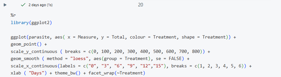
Start with my measurements on x axis are actually representing days – measures are taken in the different days and they are increasing in the timescale as they move.

I specify that measures differ on the days and also change the name of the x axis. Note, I also specify the breaks.

So by now I am quite content with my exploratory plot - the curves, the y axis, and the x axis.

I feel the plot feels kind of intuitive. Someone just by looking at it can tell that this is measuring total amount changing during the time scale.

One thing I am not a big fan of is the background, let’s fix it.

I will use theme_bw () function.

My personal taste it feels less cluttered with theme_bw ( ), i have been using that one quite a lot, but there are many themes available.

I am happy with how it is displayed in comparison to each other.

At the same time, maybe I want to take a look how it looks differing in different treatments, let’s separate it with the facet_wrap function by treatment:

Hm... If i think of it, actually each of my treatments contain 3 treatments within each other, which we call “populations”. In this case I want to define the shapes and colors within each treatment to have an own color and shape, as it is total 3 x 3 = 9 treatments, I will specify which colors I want to use.

Some color inspiration of native ones can be found here: https://r-graph-gallery.com/ggplot2-color.html

But something looks off in my plot – I can see the treatments are actually not displaying each of my datapoints, I have indicated as in positive treatment there is no highest values of my parasite load points;

We can see it in the error message.

Thus, I will specify shapes as well.

There are many shapes one can specify.

I adjusted some colors as well, so they “fit my taste” a bit better.

NOTE: this is just for the purpose of this tutorial so they look a bit nice according to my taste, I generally would advise to use some more contrasting colors for discriminating treatments and colors against each other. In my honest opinion, plots should firstly depict the message and SHOW the data or insights, and secondly look nice/presentable. Well, in this case this is not the focus.

Lastly, I don’t really like that the lines are displayed in the same colors against these all three different treatments in the blocks.

I will also make sure to specify this in the scale color manual.

Here, we have went from a rather simple plot, to an increased complexity using ggplot2.

Of course, there is always limitless ways to customize everything for example one thing i find very useful – combining plots together:

Some of the libraries I personally used before and like a lot is cowplot, patchwork.

Just for the sake of it – patchwork doesn’t come in as native in Databricks so I have to install it by myself - by simply running this.

Then I load the wanted library

Then lets try combining: I will simply adjust that certain ggplot2 belongs to one function "p1"

Another set to another function "p2"

And then at the end I will specify that I want them displayed nearby each other: "p1 + p2"

In this case the spacing was not great, but I think what could potentially work is actually placing them on top and bottom, lets try, by using the function p1 / p2

Looks promising, but I do not like the legend situation, it seems to not fully fit, maybe I will just outsource that the legends are displayed at the bottom of the plots instead:

Well, as you can see, the legends look better now.

Ideally, I would consider actually coming back to the the plot and starting to publish the legends on the initial it form of the plot itself rather than fixing it on while merging in the common plot; Maybe even do the same colors for the lines of treatments and merge the legends together.

Technically polishing of the plots can be happening forever, and there are SO many ways to do R and ggplot2. To each their own.

But likely by now, you have gotten some ideas on how to play with your data already and can continue that journey on your own.

If I want to remove my just installed package I should use this function: